import pandas as pd
import numpy as np
import matplotlib.pyplot as plt12 Pandas
Pandas is a library for storing and manipulating tabular data, or data stored in rows and columns like a spreadsheet. Pandas is a huge library with many different functions and methods, so what follows is a brief introduction to the most important functions for data management.
Note
If you encounter any part of Pandas out in the wild that you don’t see here, you can always refer to the Pandas documentation.
12.1 DataFrames and Series
Instead of normal Python lists and dictionaries, Pandas stores data in its own specialized objects. The main one is a DataFrame, which is a lot like a spreadsheet with rows and columns.
You can create a DataFrame directly with the DataFrame() class in Pandas, but it’s more likely that you’ll read in a DataFrame from a CSV or spreadsheet file. First you must import the library, and it’s a good idea to import the numpy and matplotlib libraries as well.
Tip
Numpy is a Python library for efficiently handling arrays and matrices of numbers. Matplotlib is a Python library for creating data visualizations. Pandas uses both under the hood to run background operations. You usually won’t need to use them directly, but it’s good to have them imported to avoid any mysterious errors.
Now you can use the read_csv() function to read in a comma-separated value (CSV) spreadsheet file. You must put the name of this file in quotes, and the file should be in the same directory as your Jupyter notebook (or else you should include a full path). The read_csv() function will also accept a URL that points to a CSV file online.
For this example, we’ll use the file mpg.csv which comes from R’s ggplot2 library.
mpg = pd.read_csv("../data/mpg.csv")
mpg| manufacturer | model | displ | year | cyl | trans | drv | cty | hwy | fl | class | |
|---|---|---|---|---|---|---|---|---|---|---|---|
| 0 | audi | a4 | 1.8 | 1999 | 4 | auto(l5) | f | 18 | 29 | p | compact |
| 1 | audi | a4 | 1.8 | 1999 | 4 | manual(m5) | f | 21 | 29 | p | compact |
| 2 | audi | a4 | 2.0 | 2008 | 4 | manual(m6) | f | 20 | 31 | p | compact |
| 3 | audi | a4 | 2.0 | 2008 | 4 | auto(av) | f | 21 | 30 | p | compact |
| 4 | audi | a4 | 2.8 | 1999 | 6 | auto(l5) | f | 16 | 26 | p | compact |
| ... | ... | ... | ... | ... | ... | ... | ... | ... | ... | ... | ... |
| 229 | volkswagen | passat | 2.0 | 2008 | 4 | auto(s6) | f | 19 | 28 | p | midsize |
| 230 | volkswagen | passat | 2.0 | 2008 | 4 | manual(m6) | f | 21 | 29 | p | midsize |
| 231 | volkswagen | passat | 2.8 | 1999 | 6 | auto(l5) | f | 16 | 26 | p | midsize |
| 232 | volkswagen | passat | 2.8 | 1999 | 6 | manual(m5) | f | 18 | 26 | p | midsize |
| 233 | volkswagen | passat | 3.6 | 2008 | 6 | auto(s6) | f | 17 | 26 | p | midsize |
234 rows × 11 columns
Warning
Jupyter nicely formats DataFrames as tables when you type the name of a variable containing a DataFrame. But if you use the print() function, it won’t display as well.
You can get basic information about your DataFrames columns using the .info() method.
mpg.info()<class 'pandas.DataFrame'>
RangeIndex: 234 entries, 0 to 233
Data columns (total 11 columns):
# Column Non-Null Count Dtype
--- ------ -------------- -----
0 manufacturer 234 non-null str
1 model 234 non-null str
2 displ 234 non-null float64
3 year 234 non-null int64
4 cyl 234 non-null int64
5 trans 234 non-null str
6 drv 234 non-null str
7 cty 234 non-null int64
8 hwy 234 non-null int64
9 fl 234 non-null str
10 class 234 non-null str
dtypes: float64(1), int64(4), str(6)
memory usage: 27.9 KBA Series is a lot like a Python list, and each column of a DataFrame is a Series. You can access the columns of a Dataframe with dot notation.
mpg.model0 a4
1 a4
2 a4
3 a4
4 a4
...
229 passat
230 passat
231 passat
232 passat
233 passat
Name: model, Length: 234, dtype: strYou can also turn a list into a Series with the Series() class.
myseries = pd.Series([5, 6, 7, 8])
myseries
0 5
1 6
2 7
3 8
dtype: int6412.2 Selecting Rows and Columns
Once you have a DataFrame, you’ll typically want to filter and select different rows or columns.
To filter specific rows, Pandas uses a bracket notation. It takes conditional statements that are similar to Python conditions.
# Get cars with fewer than 6 cylinders
four_cylinders = mpg[mpg.cyl < 6]
four_cylinders| manufacturer | model | displ | year | cyl | trans | drv | cty | hwy | fl | class | |
|---|---|---|---|---|---|---|---|---|---|---|---|
| 0 | audi | a4 | 1.8 | 1999 | 4 | auto(l5) | f | 18 | 29 | p | compact |
| 1 | audi | a4 | 1.8 | 1999 | 4 | manual(m5) | f | 21 | 29 | p | compact |
| 2 | audi | a4 | 2.0 | 2008 | 4 | manual(m6) | f | 20 | 31 | p | compact |
| 3 | audi | a4 | 2.0 | 2008 | 4 | auto(av) | f | 21 | 30 | p | compact |
| 7 | audi | a4 quattro | 1.8 | 1999 | 4 | manual(m5) | 4 | 18 | 26 | p | compact |
| ... | ... | ... | ... | ... | ... | ... | ... | ... | ... | ... | ... |
| 226 | volkswagen | new beetle | 2.5 | 2008 | 5 | auto(s6) | f | 20 | 29 | r | subcompact |
| 227 | volkswagen | passat | 1.8 | 1999 | 4 | manual(m5) | f | 21 | 29 | p | midsize |
| 228 | volkswagen | passat | 1.8 | 1999 | 4 | auto(l5) | f | 18 | 29 | p | midsize |
| 229 | volkswagen | passat | 2.0 | 2008 | 4 | auto(s6) | f | 19 | 28 | p | midsize |
| 230 | volkswagen | passat | 2.0 | 2008 | 4 | manual(m6) | f | 21 | 29 | p | midsize |
85 rows × 11 columns
You can also use the operators & (and), | (or), and ! (not) to combine conditional filters.
# Get Volkswagens and Fords
vw_ford = mpg[(mpg.manufacturer == 'volkswagen') | (mpg.manufacturer == 'ford')]
vw_ford| manufacturer | model | displ | year | cyl | trans | drv | cty | hwy | fl | class | |
|---|---|---|---|---|---|---|---|---|---|---|---|
| 74 | ford | expedition 2wd | 4.6 | 1999 | 8 | auto(l4) | r | 11 | 17 | r | suv |
| 75 | ford | expedition 2wd | 5.4 | 1999 | 8 | auto(l4) | r | 11 | 17 | r | suv |
| 76 | ford | expedition 2wd | 5.4 | 2008 | 8 | auto(l6) | r | 12 | 18 | r | suv |
| 77 | ford | explorer 4wd | 4.0 | 1999 | 6 | auto(l5) | 4 | 14 | 17 | r | suv |
| 78 | ford | explorer 4wd | 4.0 | 1999 | 6 | manual(m5) | 4 | 15 | 19 | r | suv |
| 79 | ford | explorer 4wd | 4.0 | 1999 | 6 | auto(l5) | 4 | 14 | 17 | r | suv |
| 80 | ford | explorer 4wd | 4.0 | 2008 | 6 | auto(l5) | 4 | 13 | 19 | r | suv |
| 81 | ford | explorer 4wd | 4.6 | 2008 | 8 | auto(l6) | 4 | 13 | 19 | r | suv |
| 82 | ford | explorer 4wd | 5.0 | 1999 | 8 | auto(l4) | 4 | 13 | 17 | r | suv |
| 83 | ford | f150 pickup 4wd | 4.2 | 1999 | 6 | auto(l4) | 4 | 14 | 17 | r | pickup |
| 84 | ford | f150 pickup 4wd | 4.2 | 1999 | 6 | manual(m5) | 4 | 14 | 17 | r | pickup |
| 85 | ford | f150 pickup 4wd | 4.6 | 1999 | 8 | manual(m5) | 4 | 13 | 16 | r | pickup |
| 86 | ford | f150 pickup 4wd | 4.6 | 1999 | 8 | auto(l4) | 4 | 13 | 16 | r | pickup |
| 87 | ford | f150 pickup 4wd | 4.6 | 2008 | 8 | auto(l4) | 4 | 13 | 17 | r | pickup |
| 88 | ford | f150 pickup 4wd | 5.4 | 1999 | 8 | auto(l4) | 4 | 11 | 15 | r | pickup |
| 89 | ford | f150 pickup 4wd | 5.4 | 2008 | 8 | auto(l4) | 4 | 13 | 17 | r | pickup |
| 90 | ford | mustang | 3.8 | 1999 | 6 | manual(m5) | r | 18 | 26 | r | subcompact |
| 91 | ford | mustang | 3.8 | 1999 | 6 | auto(l4) | r | 18 | 25 | r | subcompact |
| 92 | ford | mustang | 4.0 | 2008 | 6 | manual(m5) | r | 17 | 26 | r | subcompact |
| 93 | ford | mustang | 4.0 | 2008 | 6 | auto(l5) | r | 16 | 24 | r | subcompact |
| 94 | ford | mustang | 4.6 | 1999 | 8 | auto(l4) | r | 15 | 21 | r | subcompact |
| 95 | ford | mustang | 4.6 | 1999 | 8 | manual(m5) | r | 15 | 22 | r | subcompact |
| 96 | ford | mustang | 4.6 | 2008 | 8 | manual(m5) | r | 15 | 23 | r | subcompact |
| 97 | ford | mustang | 4.6 | 2008 | 8 | auto(l5) | r | 15 | 22 | r | subcompact |
| 98 | ford | mustang | 5.4 | 2008 | 8 | manual(m6) | r | 14 | 20 | p | subcompact |
| 207 | volkswagen | gti | 2.0 | 1999 | 4 | manual(m5) | f | 21 | 29 | r | compact |
| 208 | volkswagen | gti | 2.0 | 1999 | 4 | auto(l4) | f | 19 | 26 | r | compact |
| 209 | volkswagen | gti | 2.0 | 2008 | 4 | manual(m6) | f | 21 | 29 | p | compact |
| 210 | volkswagen | gti | 2.0 | 2008 | 4 | auto(s6) | f | 22 | 29 | p | compact |
| 211 | volkswagen | gti | 2.8 | 1999 | 6 | manual(m5) | f | 17 | 24 | r | compact |
| 212 | volkswagen | jetta | 1.9 | 1999 | 4 | manual(m5) | f | 33 | 44 | d | compact |
| 213 | volkswagen | jetta | 2.0 | 1999 | 4 | manual(m5) | f | 21 | 29 | r | compact |
| 214 | volkswagen | jetta | 2.0 | 1999 | 4 | auto(l4) | f | 19 | 26 | r | compact |
| 215 | volkswagen | jetta | 2.0 | 2008 | 4 | auto(s6) | f | 22 | 29 | p | compact |
| 216 | volkswagen | jetta | 2.0 | 2008 | 4 | manual(m6) | f | 21 | 29 | p | compact |
| 217 | volkswagen | jetta | 2.5 | 2008 | 5 | auto(s6) | f | 21 | 29 | r | compact |
| 218 | volkswagen | jetta | 2.5 | 2008 | 5 | manual(m5) | f | 21 | 29 | r | compact |
| 219 | volkswagen | jetta | 2.8 | 1999 | 6 | auto(l4) | f | 16 | 23 | r | compact |
| 220 | volkswagen | jetta | 2.8 | 1999 | 6 | manual(m5) | f | 17 | 24 | r | compact |
| 221 | volkswagen | new beetle | 1.9 | 1999 | 4 | manual(m5) | f | 35 | 44 | d | subcompact |
| 222 | volkswagen | new beetle | 1.9 | 1999 | 4 | auto(l4) | f | 29 | 41 | d | subcompact |
| 223 | volkswagen | new beetle | 2.0 | 1999 | 4 | manual(m5) | f | 21 | 29 | r | subcompact |
| 224 | volkswagen | new beetle | 2.0 | 1999 | 4 | auto(l4) | f | 19 | 26 | r | subcompact |
| 225 | volkswagen | new beetle | 2.5 | 2008 | 5 | manual(m5) | f | 20 | 28 | r | subcompact |
| 226 | volkswagen | new beetle | 2.5 | 2008 | 5 | auto(s6) | f | 20 | 29 | r | subcompact |
| 227 | volkswagen | passat | 1.8 | 1999 | 4 | manual(m5) | f | 21 | 29 | p | midsize |
| 228 | volkswagen | passat | 1.8 | 1999 | 4 | auto(l5) | f | 18 | 29 | p | midsize |
| 229 | volkswagen | passat | 2.0 | 2008 | 4 | auto(s6) | f | 19 | 28 | p | midsize |
| 230 | volkswagen | passat | 2.0 | 2008 | 4 | manual(m6) | f | 21 | 29 | p | midsize |
| 231 | volkswagen | passat | 2.8 | 1999 | 6 | auto(l5) | f | 16 | 26 | p | midsize |
| 232 | volkswagen | passat | 2.8 | 1999 | 6 | manual(m5) | f | 18 | 26 | p | midsize |
| 233 | volkswagen | passat | 3.6 | 2008 | 6 | auto(s6) | f | 17 | 26 | p | midsize |
You can use a double bracket notation to select a subset of columns.
Tip
Using single brackets or dot notation will get you a single column as a Series.
class_cty_hwy = mpg[["class", "cty", "hwy"]]
class_cty_hwy| class | cty | hwy | |
|---|---|---|---|
| 0 | compact | 18 | 29 |
| 1 | compact | 21 | 29 |
| 2 | compact | 20 | 31 |
| 3 | compact | 21 | 30 |
| 4 | compact | 16 | 26 |
| ... | ... | ... | ... |
| 229 | midsize | 19 | 28 |
| 230 | midsize | 21 | 29 |
| 231 | midsize | 16 | 26 |
| 232 | midsize | 18 | 26 |
| 233 | midsize | 17 | 26 |
234 rows × 3 columns
12.3 Data Wrangling
In addtion to selecting rows and columns from DataFrames, you can also use Pandas to do a wide variety of data transformations.
12.3.1 Sorting
mpg.sort_values("year", ascending=False)| manufacturer | model | displ | year | cyl | trans | drv | cty | hwy | fl | class | |
|---|---|---|---|---|---|---|---|---|---|---|---|
| 117 | hyundai | tiburon | 2.0 | 2008 | 4 | manual(m5) | f | 20 | 28 | r | subcompact |
| 120 | hyundai | tiburon | 2.7 | 2008 | 6 | manual(m6) | f | 16 | 24 | r | subcompact |
| 122 | jeep | grand cherokee 4wd | 3.0 | 2008 | 6 | auto(l5) | 4 | 17 | 22 | d | suv |
| 123 | jeep | grand cherokee 4wd | 3.7 | 2008 | 6 | auto(l5) | 4 | 15 | 19 | r | suv |
| 126 | jeep | grand cherokee 4wd | 4.7 | 2008 | 8 | auto(l5) | 4 | 9 | 12 | e | suv |
| ... | ... | ... | ... | ... | ... | ... | ... | ... | ... | ... | ... |
| 130 | land rover | range rover | 4.0 | 1999 | 8 | auto(l4) | 4 | 11 | 15 | p | suv |
| 50 | dodge | dakota pickup 4wd | 3.9 | 1999 | 6 | auto(l4) | 4 | 13 | 17 | r | pickup |
| 51 | dodge | dakota pickup 4wd | 3.9 | 1999 | 6 | manual(m5) | 4 | 14 | 17 | r | pickup |
| 125 | jeep | grand cherokee 4wd | 4.7 | 1999 | 8 | auto(l4) | 4 | 14 | 17 | r | suv |
| 0 | audi | a4 | 1.8 | 1999 | 4 | auto(l5) | f | 18 | 29 | p | compact |
234 rows × 11 columns
12.3.2 Counting
mpg.value_counts("manufacturer")manufacturer
dodge 37
toyota 34
volkswagen 27
ford 25
chevrolet 19
audi 18
hyundai 14
subaru 14
nissan 13
honda 9
jeep 8
pontiac 5
land rover 4
mercury 4
lincoln 3
Name: count, dtype: int6412.3.3 Renaming Columns
# Note the use of a Python dictionary as this method's argument
mpg = mpg.rename({"cty":"city", "hwy": "highway"})
mpg| manufacturer | model | displ | year | cyl | trans | drv | cty | hwy | fl | class | |
|---|---|---|---|---|---|---|---|---|---|---|---|
| 0 | audi | a4 | 1.8 | 1999 | 4 | auto(l5) | f | 18 | 29 | p | compact |
| 1 | audi | a4 | 1.8 | 1999 | 4 | manual(m5) | f | 21 | 29 | p | compact |
| 2 | audi | a4 | 2.0 | 2008 | 4 | manual(m6) | f | 20 | 31 | p | compact |
| 3 | audi | a4 | 2.0 | 2008 | 4 | auto(av) | f | 21 | 30 | p | compact |
| 4 | audi | a4 | 2.8 | 1999 | 6 | auto(l5) | f | 16 | 26 | p | compact |
| ... | ... | ... | ... | ... | ... | ... | ... | ... | ... | ... | ... |
| 229 | volkswagen | passat | 2.0 | 2008 | 4 | auto(s6) | f | 19 | 28 | p | midsize |
| 230 | volkswagen | passat | 2.0 | 2008 | 4 | manual(m6) | f | 21 | 29 | p | midsize |
| 231 | volkswagen | passat | 2.8 | 1999 | 6 | auto(l5) | f | 16 | 26 | p | midsize |
| 232 | volkswagen | passat | 2.8 | 1999 | 6 | manual(m5) | f | 18 | 26 | p | midsize |
| 233 | volkswagen | passat | 3.6 | 2008 | 6 | auto(s6) | f | 17 | 26 | p | midsize |
234 rows × 11 columns
12.3.4 Create new columns
You can use assign() to create new columns based on existing ones.
mpg = mpg.assign(displ_per_cyl = mpg.displ/mpg.cyl)
mpg| manufacturer | model | displ | year | cyl | trans | drv | cty | hwy | fl | class | displ_per_cyl | |
|---|---|---|---|---|---|---|---|---|---|---|---|---|
| 0 | audi | a4 | 1.8 | 1999 | 4 | auto(l5) | f | 18 | 29 | p | compact | 0.450000 |
| 1 | audi | a4 | 1.8 | 1999 | 4 | manual(m5) | f | 21 | 29 | p | compact | 0.450000 |
| 2 | audi | a4 | 2.0 | 2008 | 4 | manual(m6) | f | 20 | 31 | p | compact | 0.500000 |
| 3 | audi | a4 | 2.0 | 2008 | 4 | auto(av) | f | 21 | 30 | p | compact | 0.500000 |
| 4 | audi | a4 | 2.8 | 1999 | 6 | auto(l5) | f | 16 | 26 | p | compact | 0.466667 |
| ... | ... | ... | ... | ... | ... | ... | ... | ... | ... | ... | ... | ... |
| 229 | volkswagen | passat | 2.0 | 2008 | 4 | auto(s6) | f | 19 | 28 | p | midsize | 0.500000 |
| 230 | volkswagen | passat | 2.0 | 2008 | 4 | manual(m6) | f | 21 | 29 | p | midsize | 0.500000 |
| 231 | volkswagen | passat | 2.8 | 1999 | 6 | auto(l5) | f | 16 | 26 | p | midsize | 0.466667 |
| 232 | volkswagen | passat | 2.8 | 1999 | 6 | manual(m5) | f | 18 | 26 | p | midsize | 0.466667 |
| 233 | volkswagen | passat | 3.6 | 2008 | 6 | auto(s6) | f | 17 | 26 | p | midsize | 0.600000 |
234 rows × 12 columns
12.3.5 Grouping and Summarizing
This combines a couple functions that exist within Pandas to create summary tables.
Pandas has a wide range of summary statistics that you can apply to individual columns.
# Average city fuel efficiency
mpg.cty.mean()np.float64(16.858974358974358)# Standard deviation of highway fuel efficiency
mpg.hwy.std()np.float64(5.9546434411664455)Pandas also has a .groupby() method (which returns a generator) that groups categorical variables.
mpg.groupby("manufacturer")<pandas.api.typing.DataFrameGroupBy object at 0x114ea7b60>By itself, .groupby() doesn’t show anything. It needs to be combined with a summary statistic to create a summary table.
# Averages by manufacturer
# set `numeric_only=True` to avoid a warning
mpg.groupby("manufacturer").mean(numeric_only=True)| displ | year | cyl | cty | hwy | displ_per_cyl | |
|---|---|---|---|---|---|---|
| manufacturer | ||||||
| audi | 2.544444 | 2003.500000 | 5.222222 | 17.611111 | 26.444444 | 0.484722 |
| chevrolet | 5.063158 | 2004.684211 | 7.263158 | 15.000000 | 21.894737 | 0.686842 |
| dodge | 4.378378 | 2004.108108 | 7.081081 | 13.135135 | 17.945946 | 0.616216 |
| ford | 4.536000 | 2002.600000 | 7.200000 | 14.000000 | 19.360000 | 0.633667 |
| honda | 1.711111 | 2003.000000 | 4.000000 | 24.444444 | 32.555556 | 0.427778 |
| hyundai | 2.428571 | 2004.142857 | 4.857143 | 18.642857 | 26.857143 | 0.509524 |
| jeep | 4.575000 | 2005.750000 | 7.250000 | 13.500000 | 17.625000 | 0.627604 |
| land rover | 4.300000 | 2003.500000 | 8.000000 | 11.500000 | 16.500000 | 0.537500 |
| lincoln | 5.400000 | 2002.000000 | 8.000000 | 11.333333 | 17.000000 | 0.675000 |
| mercury | 4.400000 | 2003.500000 | 7.000000 | 13.250000 | 18.000000 | 0.633333 |
| nissan | 3.269231 | 2003.846154 | 5.538462 | 18.076923 | 24.615385 | 0.589744 |
| pontiac | 3.960000 | 2002.600000 | 6.400000 | 17.000000 | 26.400000 | 0.615833 |
| subaru | 2.457143 | 2004.142857 | 4.000000 | 19.285714 | 25.571429 | 0.614286 |
| toyota | 2.952941 | 2002.705882 | 5.117647 | 18.529412 | 24.911765 | 0.573897 |
| volkswagen | 2.255556 | 2002.666667 | 4.592593 | 20.925926 | 29.222222 | 0.491049 |
12.3.6 Dropping Null Values
For many statistical modeling tasks, you need to drop rows that contain null values. Pandas lets you do this easily with .dropna().
Note
Pandas typically stores null values as NaN, which stands for “not a number.”
# Drop any row that contains a null value in any column
mpg = mpg.dropna()
mpg| manufacturer | model | displ | year | cyl | trans | drv | cty | hwy | fl | class | displ_per_cyl | |
|---|---|---|---|---|---|---|---|---|---|---|---|---|
| 0 | audi | a4 | 1.8 | 1999 | 4 | auto(l5) | f | 18 | 29 | p | compact | 0.450000 |
| 1 | audi | a4 | 1.8 | 1999 | 4 | manual(m5) | f | 21 | 29 | p | compact | 0.450000 |
| 2 | audi | a4 | 2.0 | 2008 | 4 | manual(m6) | f | 20 | 31 | p | compact | 0.500000 |
| 3 | audi | a4 | 2.0 | 2008 | 4 | auto(av) | f | 21 | 30 | p | compact | 0.500000 |
| 4 | audi | a4 | 2.8 | 1999 | 6 | auto(l5) | f | 16 | 26 | p | compact | 0.466667 |
| ... | ... | ... | ... | ... | ... | ... | ... | ... | ... | ... | ... | ... |
| 229 | volkswagen | passat | 2.0 | 2008 | 4 | auto(s6) | f | 19 | 28 | p | midsize | 0.500000 |
| 230 | volkswagen | passat | 2.0 | 2008 | 4 | manual(m6) | f | 21 | 29 | p | midsize | 0.500000 |
| 231 | volkswagen | passat | 2.8 | 1999 | 6 | auto(l5) | f | 16 | 26 | p | midsize | 0.466667 |
| 232 | volkswagen | passat | 2.8 | 1999 | 6 | manual(m5) | f | 18 | 26 | p | midsize | 0.466667 |
| 233 | volkswagen | passat | 3.6 | 2008 | 6 | auto(s6) | f | 17 | 26 | p | midsize | 0.600000 |
234 rows × 12 columns
Warning
The mpg dataset doesn’t contain any null values, so right now this code isn’t accomplishing anything. But it will work when null values are present!
You can also drop null values from only a subset of columns.
# Drop any rows that contain null values in a subset of columns
mpg = mpg.dropna(subset=["model", "displ"])
mpg| manufacturer | model | displ | year | cyl | trans | drv | cty | hwy | fl | class | displ_per_cyl | |
|---|---|---|---|---|---|---|---|---|---|---|---|---|
| 0 | audi | a4 | 1.8 | 1999 | 4 | auto(l5) | f | 18 | 29 | p | compact | 0.450000 |
| 1 | audi | a4 | 1.8 | 1999 | 4 | manual(m5) | f | 21 | 29 | p | compact | 0.450000 |
| 2 | audi | a4 | 2.0 | 2008 | 4 | manual(m6) | f | 20 | 31 | p | compact | 0.500000 |
| 3 | audi | a4 | 2.0 | 2008 | 4 | auto(av) | f | 21 | 30 | p | compact | 0.500000 |
| 4 | audi | a4 | 2.8 | 1999 | 6 | auto(l5) | f | 16 | 26 | p | compact | 0.466667 |
| ... | ... | ... | ... | ... | ... | ... | ... | ... | ... | ... | ... | ... |
| 229 | volkswagen | passat | 2.0 | 2008 | 4 | auto(s6) | f | 19 | 28 | p | midsize | 0.500000 |
| 230 | volkswagen | passat | 2.0 | 2008 | 4 | manual(m6) | f | 21 | 29 | p | midsize | 0.500000 |
| 231 | volkswagen | passat | 2.8 | 1999 | 6 | auto(l5) | f | 16 | 26 | p | midsize | 0.466667 |
| 232 | volkswagen | passat | 2.8 | 1999 | 6 | manual(m5) | f | 18 | 26 | p | midsize | 0.466667 |
| 233 | volkswagen | passat | 3.6 | 2008 | 6 | auto(s6) | f | 17 | 26 | p | midsize | 0.600000 |
234 rows × 12 columns
12.4 Sampling
Many statistical methods, especially hypothesis tests, require you to take a random sample of your overall data. Again, Pandas provides an easy way to do this with the .sample() method.
You can take a sample of rows from an entire dataframe.
# Get 5 random rows from mpg
mpg.sample(5)| manufacturer | model | displ | year | cyl | trans | drv | cty | hwy | fl | class | displ_per_cyl | |
|---|---|---|---|---|---|---|---|---|---|---|---|---|
| 219 | volkswagen | jetta | 2.8 | 1999 | 6 | auto(l4) | f | 16 | 23 | r | compact | 0.466667 |
| 175 | toyota | 4runner 4wd | 3.4 | 1999 | 6 | auto(l4) | 4 | 15 | 19 | r | suv | 0.566667 |
| 63 | dodge | durango 4wd | 5.9 | 1999 | 8 | auto(l4) | 4 | 11 | 15 | r | suv | 0.737500 |
| 220 | volkswagen | jetta | 2.8 | 1999 | 6 | manual(m5) | f | 17 | 24 | r | compact | 0.466667 |
| 130 | land rover | range rover | 4.0 | 1999 | 8 | auto(l4) | 4 | 11 | 15 | p | suv | 0.500000 |
You can also get a sample of a specific column.
# Get 5 sample engine displacement values, as a series
mpg.displ.sample(5)
172 2.5
61 5.2
178 4.7
35 3.5
128 5.7
Name: displ, dtype: float64You can also sample with replacement. (This is also called “bootstrap sampling.”) This makes it possible to have the same value in your sample twice.
mpg.displ.sample(5, replace=True)29 5.3
162 2.5
204 3.4
80 4.0
225 2.5
Name: displ, dtype: float64Pandas will also let you get a fraction of values instead of a set number in your sample.
# Get a random sample of one twentieth the size of the dataset
mpg.sample(frac=.05)| manufacturer | model | displ | year | cyl | trans | drv | cty | hwy | fl | class | displ_per_cyl | |
|---|---|---|---|---|---|---|---|---|---|---|---|---|
| 119 | hyundai | tiburon | 2.7 | 2008 | 6 | auto(l4) | f | 17 | 24 | r | subcompact | 0.450000 |
| 128 | jeep | grand cherokee 4wd | 5.7 | 2008 | 8 | auto(l5) | 4 | 13 | 18 | r | suv | 0.712500 |
| 160 | subaru | forester awd | 2.5 | 1999 | 4 | auto(l4) | 4 | 18 | 24 | r | suv | 0.625000 |
| 157 | pontiac | grand prix | 3.8 | 2008 | 6 | auto(l4) | f | 18 | 28 | r | midsize | 0.633333 |
| 69 | dodge | ram 1500 pickup 4wd | 4.7 | 2008 | 8 | manual(m6) | 4 | 9 | 12 | e | pickup | 0.587500 |
| 10 | audi | a4 quattro | 2.0 | 2008 | 4 | auto(s6) | 4 | 19 | 27 | p | compact | 0.500000 |
| 78 | ford | explorer 4wd | 4.0 | 1999 | 6 | manual(m5) | 4 | 15 | 19 | r | suv | 0.666667 |
| 197 | toyota | corolla | 1.8 | 2008 | 4 | auto(l4) | f | 26 | 35 | r | compact | 0.450000 |
| 3 | audi | a4 | 2.0 | 2008 | 4 | auto(av) | f | 21 | 30 | p | compact | 0.500000 |
| 40 | dodge | caravan 2wd | 3.3 | 1999 | 6 | auto(l4) | f | 16 | 22 | r | minivan | 0.550000 |
| 151 | nissan | pathfinder 4wd | 3.3 | 1999 | 6 | manual(m5) | 4 | 15 | 17 | r | suv | 0.550000 |
| 31 | chevrolet | k1500 tahoe 4wd | 6.5 | 1999 | 8 | auto(l4) | 4 | 14 | 17 | d | suv | 0.812500 |
There’s one more trick you can do with sampling. Sometimes you don’t need to get a smaller random sample: instead, you just want to reshuffle every row of the dataset. You can do this by setting frac to 1. In a way, you’re taking a random sample that is 100% of the size of the dataset! (But make sure you do this without replacement.)
mpg.displ.sample(frac=1)63 5.9
11 2.8
126 4.7
168 2.5
163 2.5
...
35 3.5
111 2.4
95 4.6
195 1.8
8 1.8
Name: displ, Length: 234, dtype: float64Pandas will remember the indices in your new Series, which means if you use this reordered sample it might put things back in order for you! To avoid this, you can reset the index and drop the old labels.
mpg.displ.sample(frac=1).reset_index(drop=True)0 3.0
1 1.9
2 2.8
3 3.7
4 3.6
...
229 4.6
230 4.0
231 2.7
232 3.7
233 3.1
Name: displ, Length: 234, dtype: float6412.5 Combining Datasets
12.5.1 Stack Data with Concatenation
If you have two datasets with identical columns but different rows, you can combine or “stack” the two datasets into one.
# Let's imagine we have two datasets.
# One for manual transmission cars:

manual = pd.read_csv("../data/manual.csv")
manual| manufacturer | model | displ | year | cyl | trans | drv | cty | hwy | fl | class | |
|---|---|---|---|---|---|---|---|---|---|---|---|
| 0 | audi | a4 | 1.8 | 1999 | 4 | manual(m5) | f | 21 | 29 | p | compact |
| 1 | audi | a4 | 2.0 | 2008 | 4 | manual(m6) | f | 20 | 31 | p | compact |
| 2 | audi | a4 | 2.8 | 1999 | 6 | manual(m5) | f | 18 | 26 | p | compact |
| 3 | audi | a4 quattro | 1.8 | 1999 | 4 | manual(m5) | 4 | 18 | 26 | p | compact |
| 4 | audi | a4 quattro | 2.0 | 2008 | 4 | manual(m6) | 4 | 20 | 28 | p | compact |
| ... | ... | ... | ... | ... | ... | ... | ... | ... | ... | ... | ... |
| 72 | volkswagen | new beetle | 2.0 | 1999 | 4 | manual(m5) | f | 21 | 29 | r | subcompact |
| 73 | volkswagen | new beetle | 2.5 | 2008 | 5 | manual(m5) | f | 20 | 28 | r | subcompact |
| 74 | volkswagen | passat | 1.8 | 1999 | 4 | manual(m5) | f | 21 | 29 | p | midsize |
| 75 | volkswagen | passat | 2.0 | 2008 | 4 | manual(m6) | f | 21 | 29 | p | midsize |
| 76 | volkswagen | passat | 2.8 | 1999 | 6 | manual(m5) | f | 18 | 26 | p | midsize |
77 rows × 11 columns
# And one for automatic transmissions:
automatic = pd.read_csv("../data/automatic.csv")
automatic| manufacturer | model | displ | year | cyl | trans | drv | cty | hwy | fl | class | |
|---|---|---|---|---|---|---|---|---|---|---|---|
| 0 | audi | a4 | 1.8 | 1999 | 4 | auto(l5) | f | 18 | 29 | p | compact |
| 1 | audi | a4 | 2.0 | 2008 | 4 | auto(av) | f | 21 | 30 | p | compact |
| 2 | audi | a4 | 2.8 | 1999 | 6 | auto(l5) | f | 16 | 26 | p | compact |
| 3 | audi | a4 | 3.1 | 2008 | 6 | auto(av) | f | 18 | 27 | p | compact |
| 4 | audi | a4 quattro | 1.8 | 1999 | 4 | auto(l5) | 4 | 16 | 25 | p | compact |
| ... | ... | ... | ... | ... | ... | ... | ... | ... | ... | ... | ... |
| 152 | volkswagen | new beetle | 2.5 | 2008 | 5 | auto(s6) | f | 20 | 29 | r | subcompact |
| 153 | volkswagen | passat | 1.8 | 1999 | 4 | auto(l5) | f | 18 | 29 | p | midsize |
| 154 | volkswagen | passat | 2.0 | 2008 | 4 | auto(s6) | f | 19 | 28 | p | midsize |
| 155 | volkswagen | passat | 2.8 | 1999 | 6 | auto(l5) | f | 16 | 26 | p | midsize |
| 156 | volkswagen | passat | 3.6 | 2008 | 6 | auto(s6) | f | 17 | 26 | p | midsize |
157 rows × 11 columns
# You can combine these into one with pd.concat()

mpg_concat = pd.concat([manual, automatic])
mpg_concat| manufacturer | model | displ | year | cyl | trans | drv | cty | hwy | fl | class | |
|---|---|---|---|---|---|---|---|---|---|---|---|
| 0 | audi | a4 | 1.8 | 1999 | 4 | manual(m5) | f | 21 | 29 | p | compact |
| 1 | audi | a4 | 2.0 | 2008 | 4 | manual(m6) | f | 20 | 31 | p | compact |
| 2 | audi | a4 | 2.8 | 1999 | 6 | manual(m5) | f | 18 | 26 | p | compact |
| 3 | audi | a4 quattro | 1.8 | 1999 | 4 | manual(m5) | 4 | 18 | 26 | p | compact |
| 4 | audi | a4 quattro | 2.0 | 2008 | 4 | manual(m6) | 4 | 20 | 28 | p | compact |
| ... | ... | ... | ... | ... | ... | ... | ... | ... | ... | ... | ... |
| 152 | volkswagen | new beetle | 2.5 | 2008 | 5 | auto(s6) | f | 20 | 29 | r | subcompact |
| 153 | volkswagen | passat | 1.8 | 1999 | 4 | auto(l5) | f | 18 | 29 | p | midsize |
| 154 | volkswagen | passat | 2.0 | 2008 | 4 | auto(s6) | f | 19 | 28 | p | midsize |
| 155 | volkswagen | passat | 2.8 | 1999 | 6 | auto(l5) | f | 16 | 26 | p | midsize |
| 156 | volkswagen | passat | 3.6 | 2008 | 6 | auto(s6) | f | 17 | 26 | p | midsize |
234 rows × 11 columns
12.5.2 Switch Rows and Columns with Pivot and Melt
Sometimes your data isn’t tidy, and rows should be columns while columns should be rows. You can resolve these problems using Pandas’ “pivot” and “melt” concepts—this is similar to Pivot Tables in Excel.
# Let's imagine you have a dataset with column headings in the rows

long_mpg = pd.read_csv("../data/melted_mpg.csv")
long_mpg| manufacturer | model | year | trans | variable | value | |
|---|---|---|---|---|---|---|
| 0 | audi | a4 | 1999 | auto(l5) | displ | 1.8 |
| 1 | audi | a4 | 1999 | manual(m5) | displ | 1.8 |
| 2 | audi | a4 | 2008 | manual(m6) | displ | 2.0 |
| 3 | audi | a4 | 2008 | auto(av) | displ | 2.0 |
| 4 | audi | a4 quattro | 1999 | manual(m5) | displ | 1.8 |
| ... | ... | ... | ... | ... | ... | ... |
| 968 | volkswagen | new beetle | 2008 | auto(s6) | class | subcompact |
| 969 | volkswagen | passat | 1999 | manual(m5) | class | midsize |
| 970 | volkswagen | passat | 1999 | auto(l5) | class | midsize |
| 971 | volkswagen | passat | 2008 | auto(s6) | class | midsize |
| 972 | volkswagen | passat | 2008 | manual(m6) | class | midsize |
973 rows × 6 columns
# Use pivot to turn the "variable" column into the column names
# You must specify which columns you want to retain as indices
# Make sure you add .reset_index()

pivoted_mpg = long_mpg.pivot(index=["manufacturer", "model", "year", "trans"], columns="variable", values="value").reset_index()
pivoted_mpg| variable | manufacturer | model | year | trans | class | cty | cyl | displ | drv | fl | hwy |
|---|---|---|---|---|---|---|---|---|---|---|---|
| 0 | audi | a4 | 1999 | auto(l5) | compact | 18 | 4 | 1.8 | f | p | 29 |
| 1 | audi | a4 | 1999 | manual(m5) | compact | 21 | 4 | 1.8 | f | p | 29 |
| 2 | audi | a4 | 2008 | auto(av) | compact | 21 | 4 | 2.0 | f | p | 30 |
| 3 | audi | a4 | 2008 | manual(m6) | compact | 20 | 4 | 2.0 | f | p | 31 |
| 4 | audi | a4 quattro | 1999 | auto(l5) | compact | 16 | 4 | 1.8 | 4 | p | 25 |
| ... | ... | ... | ... | ... | ... | ... | ... | ... | ... | ... | ... |
| 134 | volkswagen | new beetle | 2008 | manual(m5) | subcompact | 20 | 5 | 2.5 | f | r | 28 |
| 135 | volkswagen | passat | 1999 | auto(l5) | midsize | 18 | 4 | 1.8 | f | p | 29 |
| 136 | volkswagen | passat | 1999 | manual(m5) | midsize | 21 | 4 | 1.8 | f | p | 29 |
| 137 | volkswagen | passat | 2008 | auto(s6) | midsize | 19 | 4 | 2.0 | f | p | 28 |
| 138 | volkswagen | passat | 2008 | manual(m6) | midsize | 21 | 4 | 2.0 | f | p | 29 |
139 rows × 11 columns
# You can use .melt() to go in the opposite direction
# Again you must specify the columns you want to keep as indices

melted_mpg = pivoted_mpg.melt(id_vars = ["manufacturer", "model", "year", "trans"])
melted_mpg| manufacturer | model | year | trans | variable | value | |
|---|---|---|---|---|---|---|
| 0 | audi | a4 | 1999 | auto(l5) | class | compact |
| 1 | audi | a4 | 1999 | manual(m5) | class | compact |
| 2 | audi | a4 | 2008 | auto(av) | class | compact |
| 3 | audi | a4 | 2008 | manual(m6) | class | compact |
| 4 | audi | a4 quattro | 1999 | auto(l5) | class | compact |
| ... | ... | ... | ... | ... | ... | ... |
| 968 | volkswagen | new beetle | 2008 | manual(m5) | hwy | 28 |
| 969 | volkswagen | passat | 1999 | auto(l5) | hwy | 29 |
| 970 | volkswagen | passat | 1999 | manual(m5) | hwy | 29 |
| 971 | volkswagen | passat | 2008 | auto(s6) | hwy | 28 |
| 972 | volkswagen | passat | 2008 | manual(m6) | hwy | 29 |
973 rows × 6 columns
12.5.3 Join Datasets with Merge
If your columns or rows don’t match exactly, you can’t use pd.concat(). But you can still combine datasets with a database-style JOIN (just like in SQL!) using the pd.merge() function.
Warning
This database-style combining of tables is really powerful, and it can get more complicated than what we have time to cover in this class. I recommend checking out McKinney Ch. 8.2 for more details, and this all is covered in much more detail in CIS 112!
# Let's assume you have a dataset without the vehicle class column

missing_mpg = pd.read_csv("../data/mpg_no_class.csv")
missing_mpg| manufacturer | model | displ | year | cyl | trans | drv | cty | hwy | fl | |
|---|---|---|---|---|---|---|---|---|---|---|
| 0 | audi | a4 | 1.8 | 1999 | 4 | auto(l5) | f | 18 | 29 | p |
| 1 | audi | a4 | 1.8 | 1999 | 4 | manual(m5) | f | 21 | 29 | p |
| 2 | audi | a4 | 2.0 | 2008 | 4 | manual(m6) | f | 20 | 31 | p |
| 3 | audi | a4 | 2.0 | 2008 | 4 | auto(av) | f | 21 | 30 | p |
| 4 | audi | a4 | 2.8 | 1999 | 6 | auto(l5) | f | 16 | 26 | p |
| ... | ... | ... | ... | ... | ... | ... | ... | ... | ... | ... |
| 229 | volkswagen | passat | 2.0 | 2008 | 4 | auto(s6) | f | 19 | 28 | p |
| 230 | volkswagen | passat | 2.0 | 2008 | 4 | manual(m6) | f | 21 | 29 | p |
| 231 | volkswagen | passat | 2.8 | 1999 | 6 | auto(l5) | f | 16 | 26 | p |
| 232 | volkswagen | passat | 2.8 | 1999 | 6 | manual(m5) | f | 18 | 26 | p |
| 233 | volkswagen | passat | 3.6 | 2008 | 6 | auto(s6) | f | 17 | 26 | p |
234 rows × 10 columns
# And you also have a dataset (with fewer rows) that has
# class info for each make and year of vehicle

class_mpg = pd.read_csv("../data/mpg_class.csv")
class_mpg| manufacturer | model | year | class | |
|---|---|---|---|---|
| 0 | audi | a4 | 1999 | compact |
| 1 | audi | a4 | 2008 | compact |
| 2 | audi | a4 quattro | 1999 | compact |
| 3 | audi | a4 quattro | 2008 | compact |
| 4 | audi | a6 quattro | 1999 | midsize |
| ... | ... | ... | ... | ... |
| 71 | volkswagen | jetta | 2008 | compact |
| 72 | volkswagen | new beetle | 1999 | subcompact |
| 73 | volkswagen | new beetle | 2008 | subcompact |
| 74 | volkswagen | passat | 1999 | midsize |
| 75 | volkswagen | passat | 2008 | midsize |
76 rows × 4 columns
# You can add the class column to your dataframe using merge

merged_mpg = pd.merge(missing_mpg, class_mpg, how="left", on=["manufacturer", "model", "year"])
merged_mpg| manufacturer | model | displ | year | cyl | trans | drv | cty | hwy | fl | class | |
|---|---|---|---|---|---|---|---|---|---|---|---|
| 0 | audi | a4 | 1.8 | 1999 | 4 | auto(l5) | f | 18 | 29 | p | compact |
| 1 | audi | a4 | 1.8 | 1999 | 4 | manual(m5) | f | 21 | 29 | p | compact |
| 2 | audi | a4 | 2.0 | 2008 | 4 | manual(m6) | f | 20 | 31 | p | compact |
| 3 | audi | a4 | 2.0 | 2008 | 4 | auto(av) | f | 21 | 30 | p | compact |
| 4 | audi | a4 | 2.8 | 1999 | 6 | auto(l5) | f | 16 | 26 | p | compact |
| ... | ... | ... | ... | ... | ... | ... | ... | ... | ... | ... | ... |
| 229 | volkswagen | passat | 2.0 | 2008 | 4 | auto(s6) | f | 19 | 28 | p | midsize |
| 230 | volkswagen | passat | 2.0 | 2008 | 4 | manual(m6) | f | 21 | 29 | p | midsize |
| 231 | volkswagen | passat | 2.8 | 1999 | 6 | auto(l5) | f | 16 | 26 | p | midsize |
| 232 | volkswagen | passat | 2.8 | 1999 | 6 | manual(m5) | f | 18 | 26 | p | midsize |
| 233 | volkswagen | passat | 3.6 | 2008 | 6 | auto(s6) | f | 17 | 26 | p | midsize |
234 rows × 11 columns
12.6 Data Types
Python and Pandas accommodate many different types of data, and Pandas in particular deals with a range of data types beyond what we’ve already discussed. Usually, you’re likely encounter: numerical data (integers and floats), categorical data (categories and objects), text data (objects and strings), time data (dates and times), and location data (geocoordinates).
Caution
Remember, the data types that programming languages use are not always exactly equivalent to the general data types that data scientists might recognize! You’re always trying to use a technical data type that’s the best match for the data you’re trying to store.
12.6.1 Changing Data Types
A good way to check what data types are in your data is the .info() method.
mpg.info()<class 'pandas.DataFrame'>
Index: 234 entries, 0 to 233
Data columns (total 12 columns):
# Column Non-Null Count Dtype
--- ------ -------------- -----
0 manufacturer 234 non-null str
1 model 234 non-null str
2 displ 234 non-null float64
3 year 234 non-null int64
4 cyl 234 non-null int64
5 trans 234 non-null str
6 drv 234 non-null str
7 cty 234 non-null int64
8 hwy 234 non-null int64
9 fl 234 non-null str
10 class 234 non-null str
11 displ_per_cyl 234 non-null float64
dtypes: float64(2), int64(4), str(6)
memory usage: 31.5 KBPandas tries its best to guess the correct data type when your data is being imported. It doesn’t always get things right! For example, if there’s any non-numeric character in a numeric column (like a dollar sign), it will identify that as an object rather than an int or float.
Tip
Pandas will use object for any non-numeric data it doesn’t know how to deal with. Usually, it’s fine to leave this alone for categorical data, but sometimes you will need to use the more robust Category data types that Pandas provides. This lets you label categories and deal with any numeric (ordinal) data that’s actually representing a category.
If a data type is encoded incorrectly, there are two ways to change it:
# The first way is to use the general astype function:

mpg = mpg.assign(manufacturer = mpg.manufacturer.astype("category"))
mpg.info()
<class 'pandas.DataFrame'>
Index: 234 entries, 0 to 233
Data columns (total 12 columns):
# Column Non-Null Count Dtype
--- ------ -------------- -----
0 manufacturer 234 non-null category
1 model 234 non-null str
2 displ 234 non-null float64
3 year 234 non-null int64
4 cyl 234 non-null int64
5 trans 234 non-null str
6 drv 234 non-null str
7 cty 234 non-null int64
8 hwy 234 non-null int64
9 fl 234 non-null str
10 class 234 non-null str
11 displ_per_cyl 234 non-null float64
dtypes: category(1), float64(2), int64(4), str(5)
memory usage: 28.6 KB# The second way is to use a function specific to
# convert something to a number, a date, or something else:
mpg = mpg.assign(hwy = pd.to_numeric(mpg.hwy, downcast="float"))
# The downcast='float' changes your data from an int to a float
# but you could also use this to go from an object to an int or float
mpg.info()<class 'pandas.DataFrame'>
Index: 234 entries, 0 to 233
Data columns (total 12 columns):
# Column Non-Null Count Dtype
--- ------ -------------- -----
0 manufacturer 234 non-null category
1 model 234 non-null str
2 displ 234 non-null float64
3 year 234 non-null int64
4 cyl 234 non-null int64
5 trans 234 non-null str
6 drv 234 non-null str
7 cty 234 non-null int64
8 hwy 234 non-null float32
9 fl 234 non-null str
10 class 234 non-null str
11 displ_per_cyl 234 non-null float64
dtypes: category(1), float32(1), float64(2), int64(3), str(5)
memory usage: 27.7 KB
Important
Converting data from one data type to another will sometimes change the data itself. Make sure to be aware of the changes you’re making! For example, changing from a float to an int might round your data to the nearest whole number.
12.6.2 Dates and Times
The datetime data types in Python record years, months, days, hours, minutes, and seconds as distinct parts of a single cell of data. Pandas has many different functions and methods for dealing with time data. A datetime is a special type of numeric data that is usually not automatically detected by Pandas.
In the mpg data, you can change the year column to a datetime:
# You must specify the format of the date or time in the existing data
# For example: "%m-%d-%Y" would be the format "05-30-2025"

mpg = mpg.assign(year = pd.to_datetime(mpg.year, format="%Y"))
mpg| manufacturer | model | displ | year | cyl | trans | drv | cty | hwy | fl | class | displ_per_cyl | |
|---|---|---|---|---|---|---|---|---|---|---|---|---|
| 0 | audi | a4 | 1.8 | 1999-01-01 | 4 | auto(l5) | f | 18 | 29.0 | p | compact | 0.450000 |
| 1 | audi | a4 | 1.8 | 1999-01-01 | 4 | manual(m5) | f | 21 | 29.0 | p | compact | 0.450000 |
| 2 | audi | a4 | 2.0 | 2008-01-01 | 4 | manual(m6) | f | 20 | 31.0 | p | compact | 0.500000 |
| 3 | audi | a4 | 2.0 | 2008-01-01 | 4 | auto(av) | f | 21 | 30.0 | p | compact | 0.500000 |
| 4 | audi | a4 | 2.8 | 1999-01-01 | 6 | auto(l5) | f | 16 | 26.0 | p | compact | 0.466667 |
| ... | ... | ... | ... | ... | ... | ... | ... | ... | ... | ... | ... | ... |
| 229 | volkswagen | passat | 2.0 | 2008-01-01 | 4 | auto(s6) | f | 19 | 28.0 | p | midsize | 0.500000 |
| 230 | volkswagen | passat | 2.0 | 2008-01-01 | 4 | manual(m6) | f | 21 | 29.0 | p | midsize | 0.500000 |
| 231 | volkswagen | passat | 2.8 | 1999-01-01 | 6 | auto(l5) | f | 16 | 26.0 | p | midsize | 0.466667 |
| 232 | volkswagen | passat | 2.8 | 1999-01-01 | 6 | manual(m5) | f | 18 | 26.0 | p | midsize | 0.466667 |
| 233 | volkswagen | passat | 3.6 | 2008-01-01 | 6 | auto(s6) | f | 17 | 26.0 | p | midsize | 0.600000 |
234 rows × 12 columns
Now the year column is a formal datetime. Because we didn’t have information on the day and month, it automatically assigned the dates to January 1st.
To access specific parts of a datetime object, you can use the dt namespace.
# Get just the year

mpg.year.dt.year
0 1999
1 1999
2 2008
3 2008
4 1999
...
229 2008
230 2008
231 1999
232 1999
233 2008
Name: year, Length: 234, dtype: int32# Get just the month
mpg.year.dt.month0 1
1 1
2 1
3 1
4 1
..
229 1
230 1
231 1
232 1
233 1
Name: year, Length: 234, dtype: int32
Note
Datetimes are commonly used to create time series graphs and analyze other changes over time (see the Altair Guide for more on this). When dealing with a machine learning model, you might need to convert a datetime back to a numeric value to get it to work properly. You can get information on these uses and many more in the Pandas documentation.
12.6.3 Text Data and Strings
Text data is distinct from categorical data. Though nominal categories often exist in the form of text, there are lots of text data (names and IDs, longer descriptions, even whole novels!) that aren’t categories.
Like with datetime data, Pandas lets you work with its string objects through a str namespace. This lets you manipulate strings (split them, concatenate them, replace them, and more) just like you would in Python.
Tip
We’ll only show a brief example here. The main place to find information about how to work with text in Pandas is on the Text Data documentation page.
In the mpg dataset, the trans (short for transmission) column includes two pieces of information. You can use the str namespace to separate this info into two columns.
First you can see what the split will look like:
# Split on the open paranthesis to get the two parts you need
mpg.trans.str.split("(")
0 [auto, l5)]
1 [manual, m5)]
2 [manual, m6)]
3 [auto, av)]
4 [auto, l5)]
...
229 [auto, s6)]
230 [manual, m6)]
231 [auto, l5)]
232 [manual, m5)]
233 [auto, s6)]
Name: trans, Length: 234, dtype: objectThen you can get each part of the string and assign it to new columns. (You don’t need to display the above part every time.)
# Note we can use assign to define columns for each part of the split
# Every time we manipulate a string
mpg = mpg.assign(
    trans = mpg.trans.str.split("(").str[0],
    transmission_full = mpg.trans.str.split("(").str[1]
)
mpg| manufacturer | model | displ | year | cyl | trans | drv | cty | hwy | fl | class | displ_per_cyl | transmission_full | |
|---|---|---|---|---|---|---|---|---|---|---|---|---|---|
| 0 | audi | a4 | 1.8 | 1999-01-01 | 4 | auto | f | 18 | 29.0 | p | compact | 0.450000 | l5) |
| 1 | audi | a4 | 1.8 | 1999-01-01 | 4 | manual | f | 21 | 29.0 | p | compact | 0.450000 | m5) |
| 2 | audi | a4 | 2.0 | 2008-01-01 | 4 | manual | f | 20 | 31.0 | p | compact | 0.500000 | m6) |
| 3 | audi | a4 | 2.0 | 2008-01-01 | 4 | auto | f | 21 | 30.0 | p | compact | 0.500000 | av) |
| 4 | audi | a4 | 2.8 | 1999-01-01 | 6 | auto | f | 16 | 26.0 | p | compact | 0.466667 | l5) |
| ... | ... | ... | ... | ... | ... | ... | ... | ... | ... | ... | ... | ... | ... |
| 229 | volkswagen | passat | 2.0 | 2008-01-01 | 4 | auto | f | 19 | 28.0 | p | midsize | 0.500000 | s6) |
| 230 | volkswagen | passat | 2.0 | 2008-01-01 | 4 | manual | f | 21 | 29.0 | p | midsize | 0.500000 | m6) |
| 231 | volkswagen | passat | 2.8 | 1999-01-01 | 6 | auto | f | 16 | 26.0 | p | midsize | 0.466667 | l5) |
| 232 | volkswagen | passat | 2.8 | 1999-01-01 | 6 | manual | f | 18 | 26.0 | p | midsize | 0.466667 | m5) |
| 233 | volkswagen | passat | 3.6 | 2008-01-01 | 6 | auto | f | 17 | 26.0 | p | midsize | 0.600000 | s6) |
234 rows × 13 columns
Then you can clean up the resulting new column using the .strip() method:
# The .strip() method removes text from the beginning or end of a string
# Use .replace() if you want to remove something from anywhere in a string
mpg = mpg.assign(transmission_full = mpg.transmission_full.str.strip(")"))
mpg| manufacturer | model | displ | year | cyl | trans | drv | cty | hwy | fl | class | displ_per_cyl | transmission_full | |
|---|---|---|---|---|---|---|---|---|---|---|---|---|---|
| 0 | audi | a4 | 1.8 | 1999-01-01 | 4 | auto | f | 18 | 29.0 | p | compact | 0.450000 | l5 |
| 1 | audi | a4 | 1.8 | 1999-01-01 | 4 | manual | f | 21 | 29.0 | p | compact | 0.450000 | m5 |
| 2 | audi | a4 | 2.0 | 2008-01-01 | 4 | manual | f | 20 | 31.0 | p | compact | 0.500000 | m6 |
| 3 | audi | a4 | 2.0 | 2008-01-01 | 4 | auto | f | 21 | 30.0 | p | compact | 0.500000 | av |
| 4 | audi | a4 | 2.8 | 1999-01-01 | 6 | auto | f | 16 | 26.0 | p | compact | 0.466667 | l5 |
| ... | ... | ... | ... | ... | ... | ... | ... | ... | ... | ... | ... | ... | ... |
| 229 | volkswagen | passat | 2.0 | 2008-01-01 | 4 | auto | f | 19 | 28.0 | p | midsize | 0.500000 | s6 |
| 230 | volkswagen | passat | 2.0 | 2008-01-01 | 4 | manual | f | 21 | 29.0 | p | midsize | 0.500000 | m6 |
| 231 | volkswagen | passat | 2.8 | 1999-01-01 | 6 | auto | f | 16 | 26.0 | p | midsize | 0.466667 | l5 |
| 232 | volkswagen | passat | 2.8 | 1999-01-01 | 6 | manual | f | 18 | 26.0 | p | midsize | 0.466667 | m5 |
| 233 | volkswagen | passat | 3.6 | 2008-01-01 | 6 | auto | f | 17 | 26.0 | p | midsize | 0.600000 | s6 |
234 rows × 13 columns
12.6.4 Location Data
If your dataset has latitude and longitude values, or even specific place names, then you might be dealing with geospatial data. Geospatial data needs specialized tools, and GIS (Geographic Information Systems) is its own subfield of data science.
Important
If your data has only location names (or addresses) and you want to retrieve exact geocoordinates (latitude and longitude), you will need to use a process called geocoding which is built into many of the tools introduced in this section.
Tip
Let’s use Geopandas to look at an example of data about airports. First you should import the necessary libraries: geopandas for location data analysis and vega_datasets to get some sample data.
import geopandas
from vega_datasets import data
# Read in the sample airports data
airports = data.airports()
airports| iata | name | city | state | country | latitude | longitude | |
|---|---|---|---|---|---|---|---|
| 0 | 00M | Thigpen | Bay Springs | MS | USA | 31.953765 | -89.234505 |
| 1 | 00R | Livingston Municipal | Livingston | TX | USA | 30.685861 | -95.017928 |
| 2 | 00V | Meadow Lake | Colorado Springs | CO | USA | 38.945749 | -104.569893 |
| 3 | 01G | Perry-Warsaw | Perry | NY | USA | 42.741347 | -78.052081 |
| 4 | 01J | Hilliard Airpark | Hilliard | FL | USA | 30.688012 | -81.905944 |
| ... | ... | ... | ... | ... | ... | ... | ... |
| 3371 | ZEF | Elkin Municipal | Elkin | NC | USA | 36.280024 | -80.786069 |
| 3372 | ZER | Schuylkill Cty/Joe Zerbey | Pottsville | PA | USA | 40.706449 | -76.373147 |
| 3373 | ZPH | Zephyrhills Municipal | Zephyrhills | FL | USA | 28.228065 | -82.155916 |
| 3374 | ZUN | Black Rock | Zuni | NM | USA | 35.083227 | -108.791777 |
| 3375 | ZZV | Zanesville Municipal | Zanesville | OH | USA | 39.944458 | -81.892105 |
3376 rows × 7 columns
Once you have the airports data, you can create a “GeoDataFrame” that takes the latitude and longitude columns as points.
gdf = geopandas.GeoDataFrame(
    airports, geometry=geopandas.points_from_xy(airports.longitude, airports.latitude), crs="EPSG:4326"
)
gdf| iata | name | city | state | country | latitude | longitude | geometry | |
|---|---|---|---|---|---|---|---|---|
| 0 | 00M | Thigpen | Bay Springs | MS | USA | 31.953765 | -89.234505 | POINT (-89.2345 31.95376) |
| 1 | 00R | Livingston Municipal | Livingston | TX | USA | 30.685861 | -95.017928 | POINT (-95.01793 30.68586) |
| 2 | 00V | Meadow Lake | Colorado Springs | CO | USA | 38.945749 | -104.569893 | POINT (-104.56989 38.94575) |
| 3 | 01G | Perry-Warsaw | Perry | NY | USA | 42.741347 | -78.052081 | POINT (-78.05208 42.74135) |
| 4 | 01J | Hilliard Airpark | Hilliard | FL | USA | 30.688012 | -81.905944 | POINT (-81.90594 30.68801) |
| ... | ... | ... | ... | ... | ... | ... | ... | ... |
| 3371 | ZEF | Elkin Municipal | Elkin | NC | USA | 36.280024 | -80.786069 | POINT (-80.78607 36.28002) |
| 3372 | ZER | Schuylkill Cty/Joe Zerbey | Pottsville | PA | USA | 40.706449 | -76.373147 | POINT (-76.37315 40.70645) |
| 3373 | ZPH | Zephyrhills Municipal | Zephyrhills | FL | USA | 28.228065 | -82.155916 | POINT (-82.15592 28.22806) |
| 3374 | ZUN | Black Rock | Zuni | NM | USA | 35.083227 | -108.791777 | POINT (-108.79178 35.08323) |
| 3375 | ZZV | Zanesville Municipal | Zanesville | OH | USA | 39.944458 | -81.892105 | POINT (-81.89211 39.94446) |
3376 rows × 8 columns
Now that you have a GeoDataFrame with a geometry column, you can use it any number of ways. You could find the distance between Pittsburgh’s airport and any other.
# To get distances in meters, you must use .to_crs() to convert to
# a meter-based coordinate system

# First get the location of Pittsburgh International Airport
PIT_location = gdf[gdf.iata=="PIT"].geometry.to_crs(10598).iloc[0]

# Then use the geopandas distance method to add a new column
gdf = gdf.assign(distance_from_PIT = gdf["geometry"].to_crs(10598).distance(PIT_location))

# Sort to see the closes and farthest airports
gdf.sort_values("distance_from_PIT", ascending=False)| iata | name | city | state | country | latitude | longitude | geometry | distance_from_PIT | |
|---|---|---|---|---|---|---|---|---|---|
| 2794 | ROP | Prachinburi | NaN | NaN | Thailand | 14.078333 | 101.378334 | POINT (101.37833 14.07833) | 1.212380e+07 |
| 2795 | ROR | Babelthoup/Koror | NaN | NaN | Palau | 7.367222 | 134.544167 | POINT (134.54417 7.36722) | 1.202162e+07 |
| 3355 | YAP | Yap International | NaN | NaN | Federated States of Micronesia | 9.516700 | 138.100000 | POINT (138.1 9.5167) | 1.177099e+07 |
| 3001 | SPN | Tinian International Airport | NaN | NaN | N Mariana Islands | 14.996111 | 145.621384 | POINT (145.62138 14.99611) | 1.114018e+07 |
| 2659 | PPG | Pago Pago International | Pago Pago | AS | USA | 14.331023 | -170.710526 | POINT (-170.71053 14.33102) | 8.644101e+06 |
| ... | ... | ... | ... | ... | ... | ... | ... | ... | ... |
| 721 | 9G1 | West Penn | Tarentum | PA | USA | 40.604233 | -79.820606 | POINT (-79.82061 40.60423) | 3.729794e+04 |
| 683 | 8G7 | Zelienople | Zelienople | PA | USA | 40.801619 | -80.160729 | POINT (-80.16073 40.80162) | 3.516677e+04 |
| 1020 | BVI | Beaver County | Beaver Falls | PA | USA | 40.772481 | -80.391426 | POINT (-80.39143 40.77248) | 3.375847e+04 |
| 792 | AGC | Allegheny Cty | Pittsburgh | PA | USA | 40.354401 | -79.930169 | POINT (-79.93017 40.3544) | 2.955747e+04 |
| 2626 | PIT | Pittsburgh International | Pittsburgh | PA | USA | 40.491466 | -80.232871 | POINT (-80.23287 40.49147) | 0.000000e+00 |
3376 rows × 9 columns
How far is PIT from LAX?
gdf[gdf.iata == "LAX"]| iata | name | city | state | country | latitude | longitude | geometry | distance_from_PIT | |
|---|---|---|---|---|---|---|---|---|---|
| 2039 | LAX | Los Angeles International | Los Angeles | CA | USA | 33.942536 | -118.408074 | POINT (-118.40807 33.94254) | 3.440868e+06 |
You can use the same information to make an interactive map.
gdf.explore()Make this Notebook Trusted to load map: File -> Trust Notebook
12.7 Data Visualization
Pandas has many built-in functions for data visualizations. It provides an easy-to-understand interface for many of the most common graph types.
Note
The Pandas user guide has lots of detailed information about all the things you can do with this part of the library.
After importing any necessary libraries, it can be good to select a theme for your visualizations to make them as clear as possible. Tableau’s colorblind-safe theme is a good option:
plt.style.use('tableau-colorblind10')
# If you need to see all the available themes, you can run:
# plt.style.available
12.7.1 Distribution Plots
Distribution plots show frequencies of particular variables. Distribution plots with just one variable are histograms, which require “binning” numeric variables. The Y-axis in a histogram is always a count. You can create a histogram by using the .plot() method on a specific column of your dataset.
mpg.hwy.plot(
    kind="hist", # Specify what kind of plot you want
    alpha=0.5, # Make the bars slightly transparent (optional)
    title="Distribution of Highway Fuel Efficency", # Give your plot a title
    xlabel="Highway Fuel Efficiency (mpg)" # Label the x-axis
)
plt.show() # This makes sure the plot displays properly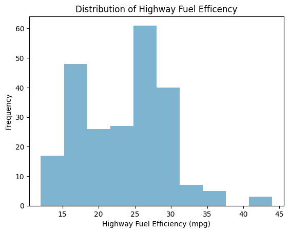
Using .pivot() (see above), you can split up the distributions by category.
mpg.pivot(columns="drv", values="hwy").plot(
    kind="hist",
    alpha=0.5,
    title="Distribution of Highway Fuel Efficiency",
    xlabel="Highway Fuel Efficiency (mpg)"
)
plt.show()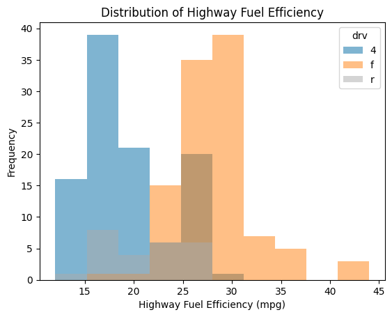
If this is hard to read, you can also split the distributions into separate subplots. This process is sometimes called faceting.
mpg.pivot(columns="drv", values="hwy").plot(
    kind="hist",
    alpha=0.5,
    title="Distribution of Highway Fuel Efficiency",
    xlabel="Highway Fuel Efficiency (mpg)",
    subplots=True
)
plt.show()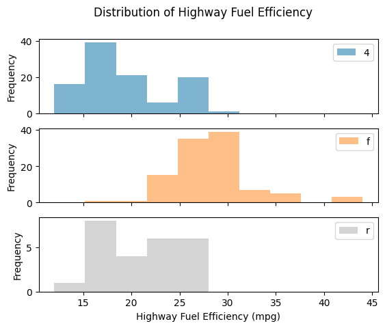
If you use a different kind of plot, you can show the distribution as a density plot instead of a histogram.
mpg.hwy.plot(
    kind="density",
    title="Density Plot of Highway Fuel Efficiency",
    xlabel="Highway Fuel Efficiency (mpg)"
)
plt.show()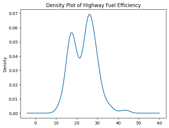
12.7.2 Category Plots
Category plots let you compare groups according to categorical variables. You can create a box plot to compare medians and distributions among groups instead of using multiple histograms. This shows a different kind of distribution, split up by category.
mpg.plot(
    kind="box",
    by="drv",
    column="hwy",
    title="Comparing Highway Fuel Efficiency Distribution by Drive Train",
    xlabel="Drive Train",
    ylabel="Highway Fuel Efficency (mpg)"
)
plt.title(None) # Remove unnecessary grouping title
plt.show()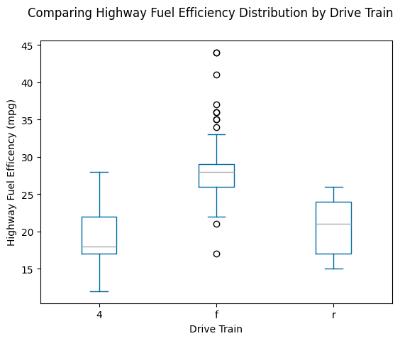
Another standard category plot is the bar plot, which usually compares means of different groups. In Pandas, we create a bar plot based on a .groupby() object, where we have already calculated the means across different groups.
mpg.groupby("drv").mean(numeric_only=True).reset_index().plot(
    kind="bar",
    y="hwy",
    x="drv",
    title="Highway Fuel Efficiency by Drive Train",
    xlabel="Drive Train",
    ylabel="Average Highway Fuel Efficiency (mpg)"
)
plt.show()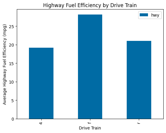
12.7.3 Relationship Plots
To show a correlation or regression between two variables, use a simple scatterplot. Scatterplots take two numerical (quantitative) variables).
mpg.plot(
    kind="scatter",
    x="displ",
    y="hwy",
    title="Comparing Highway Fuel Efficiency to Displacement",
    xlabel="Engine Displacement (liters)",
    ylabel="Highway Fuel Efficency (mpg)"
)
plt.show()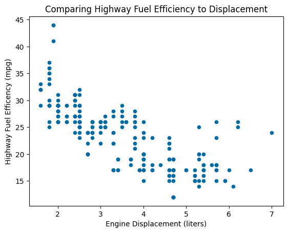
You can also create scatterplots with different colors for a categorical variable.
mpg.plot(
    kind="scatter",
    x="displ",
    y="hwy",
    c="drv",
    title="Comparing Fuel Efficiency to Displacement",
    xlabel="Engine Displacement (liters)",
    ylabel="Highway Fuel Efficency (mpg)"
)
plt.show()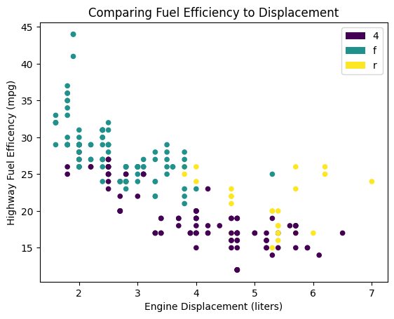
Frequently you’ll want to add a line of best fit to the graph in order to more clearly show a possible correlation. You can do that by adding a few extra lines of numpy code.
# You must drop null values first!
mpg = mpg.dropna(subset=["displ", "hwy"])
mpg.plot(
    kind="scatter",
    x="displ",
    y="hwy",
    title="Comparing Highway Fuel Efficiency to Displacement",
    xlabel="Highway Engine Displacement (liters)",
    ylabel="Fuel Efficency (mpg)"
)
# The code below creates a line of best fit and adds it to your plot
m,b = np.polyfit(x=mpg["displ"], y=mpg["hwy"], deg=1)
plt.plot(mpg.displ, m * mpg.displ + b)
plt.show()
If your scatterplot is “overplotted,” meaning that it has too many points on it to be readable, you can use a hexmap style plot to group the points into easier-to-read shaded areas.
mpg.plot(
    kind="hexbin",
    x="displ",
    y="hwy",
    gridsize=25,
    title="Comparing Highway Fuel Efficiency to Displacement",
    xlabel="Engine Displacement (liters)",
    ylabel="Highway Fuel Efficency (mpg)"
)
plt.show()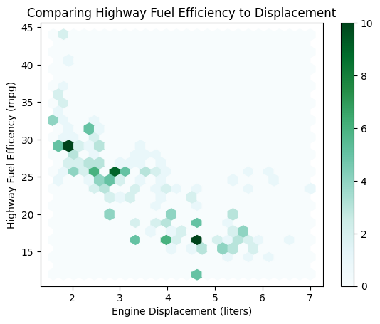
Line plots are also a kind of relationship plot. Line plots are often used with time variables, and the mpg dataset only includes two years. To make this easier to see, we’ll use Vega’s similar cars dataset. Note that you must use a .groupby() summary table to average the fuel efficiency by year, like you did for the bar plot.
from vega_datasets import data
cars = data.cars()

cars.groupby("Year").mean(numeric_only=True).reset_index().plot(
    kind="line",
    x="Year",
    y="Acceleration",
    title="Vehicle Acceleration over Time",
    ylabel="Year Car was Made",
    xlabel="Acceleration",
    legend=False
)
plt.show()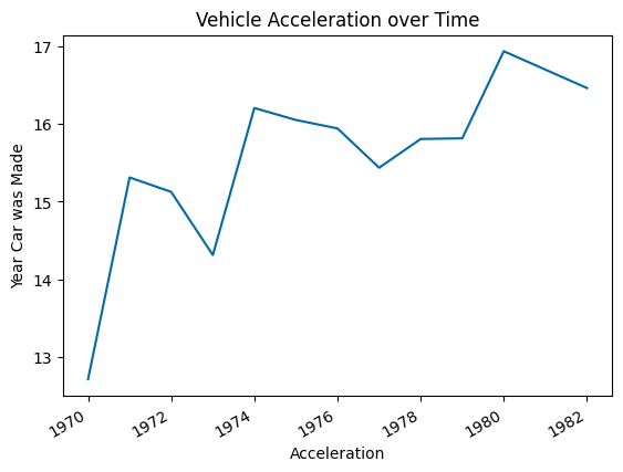
12.7.4 Special Plot Types
There are additional special plot types we will use for specific purposes. For instance, sometimes it’s necessary to show many different scatterplots at once time, using a pairplot. Pandas has a special plotting module to import for some of these special plots.
from pandas.plotting import scatter_matrixTypically you would add the above line to the very top of your code. Once that’s important, you can create the pairplot.
scatter_matrix(
    mpg,
    alpha=0.2,
    figsize=(10, 10),
    diagonal="hist"
)
plt.suptitle("Comparing all variables in MPG dataset")
plt.show()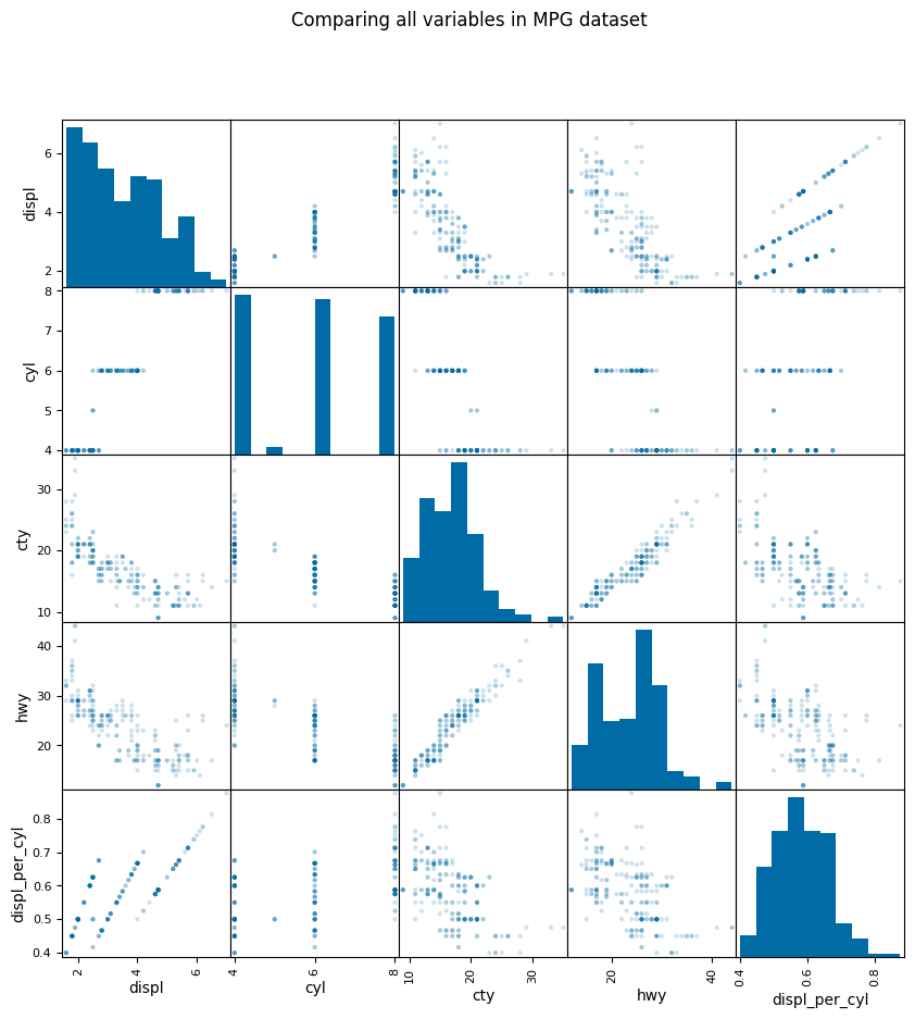
It can also be useful to add styling directly to a table. You can think of this as similar to adding colors to a spreadsheet. This is particularly useful to show a heatmap of correlation coefficients. There’s a separate section of the Pandas documentation that covers this kind of visualization.
# First create a correlation matrix
corr = mpg.corr(numeric_only=True)
# Then add the colors
corr.style.background_gradient(cmap ='coolwarm')| displ | cyl | cty | hwy | displ_per_cyl | |
|---|---|---|---|---|---|
| displ | 1.000000 | 0.930227 | -0.798524 | -0.766020 | 0.757498 |
| cyl | 0.930227 | 1.000000 | -0.805771 | -0.761912 | 0.482337 |
| cty | -0.798524 | -0.805771 | 1.000000 | 0.955916 | -0.564699 |
| hwy | -0.766020 | -0.761912 | 0.955916 | 1.000000 | -0.566210 |
| displ_per_cyl | 0.757498 | 0.482337 | -0.564699 | -0.566210 | 1.000000 |