Designed in response to a few Google Sheets-based digital humanities projects, this short guide details some ways to use Sheets to categorize and compute on the kind of data humanities scholars often collect. Though some of these functions will work in other spreadsheet programs (like Microsoft Excel and LibreOffice Calc), other functions—especially QUERY()—will only work in Google Sheets.
Sample Data
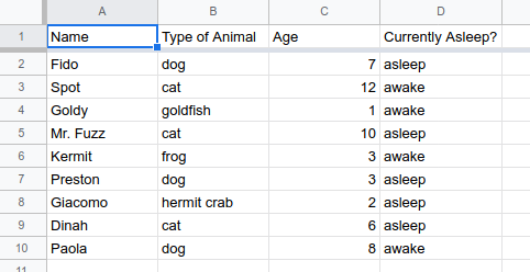
The examples below will use the same sample data, an invented spreadsheet of pet names. All of the formulas and data used in this tutorial can be found there.
The data in the spreadsheet looks like this:
Formula Basics
1) Formulas begin with =, and typing “=” in any cell will usually trigger autocomplete suggestions for different functions.
2) Formulas were designed originally to work with numerical information. If you’ve worked with them before, you’re probably familiar with SUM() and AVERAGE().
3) A full list of formulas is available using the “sigma” dropdown, to the far right of the Google Sheets toolbar. These days, formulas can be used for all sorts of things, including the kinds of data humanities scholars are often recording in spreadsheets.
4) There’s lots of Help information for every single formula, usually a click or two away once you start typing a formula.
Defining Ranges
Most functions take a range of cells as their main argument (what goes inside the parentheses). A range is two cells separated by a colon, i.e. A2:A30. Here are some examples:
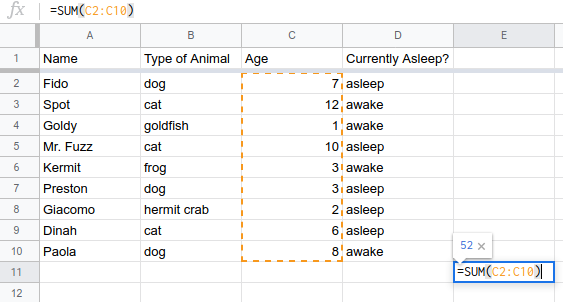
- To get the sum of the values in the first 9 rows of the third column, you would type:
=SUM(C2:C10)
This would select:
- To get the average of the values in the first 4 columns of the second row, you would type:
=AVERAGE(A2:D2)
This would select:
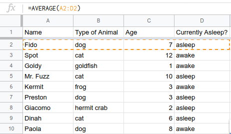
Of course, taking the average of these cells makes no sense, since not all of these values are numeric. This is just an example to see how ranges work.
- To get the maximum value of all the values in the first 9 rows of the first 4 columns (i.e., in a whole grid), you would type:
=MAX(A2:D10)
This would select:
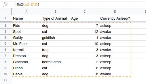
Again, this doesn’t make sense mathematically, but you can see how the range works.
Knowing how to create ranges of different sizes and shapes using this notation can really speed up your work with spreadsheets.
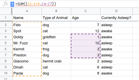
You can refer to more than one range at a time in formulae, by putting all your ranges in brackets. If you want to find the sum of column A in rows 1 through 10, but then also of column C in rows 4 through 7, you would type:
=SUM({A2:A10,C4:C7})
This would select:
Sometimes, when you copy a formula from one cell to another, the range will automatically change. (I.e. if you copy a formula from column J to column K, the spreadsheet software will assume you now care about the values in column K, rather than the ones in J.) If you want to keep some part of your range stable as you move the formula around, you can preface it with a $ sign.
The range $A1:$A10 won’t diverge from column A if you move the formula to a new column. And the range A$2:J$2 won’t switch from row 2 if you move the formula to a new row. The range $A$1:$J$10 won’t change at all no matter where you move it.
Finally, sometimes you want to select an entire column or row. You do this by omitting either the letter or number. The range A1:A will select the whole first column. The range A1:1 will select the whole first row. By this principle, you can also select an entire sheet by using the range A:Z (as long as it doesn’t have more than Z columns!).
Referencing Multiple Sheets
When collecting data, it’s often easiest to keep things straight by putting data into separate sheets. If you’re collecting data on farm animals, you might have one sheet labeled “Cows,” another for “Pigs,” and a third for “Chickens.” But when it comes time to analyze all that data, you might want to look at the same range in all three sheets.
You can refer to a different sheet by putting the sheet name with an exclamation point before the range.To get the sum of the values in the first 10 rows of the first column in the Cows sheet, you would type:
=SUM(Cows!A1:A10)
If your sheet name has a space in it, you will need to put the sheet name in quotation marks.
You can refer to the same range (or different ranges) in multiple sheets by using the same bracket notation from above. To find the sum of column A, rows 1-10 in the Cows, Pigs, and Chickens sheets, you would type:
=SUM({Cows!A1:A10, Pigs!A1:A10, Chickens!A1:A10})
If you have a lot of sheets, this can get tedious quickly. It might be easier in those cases to consolidate your data into a single sheet and refer to it all at once.
Counting
If you’re already familiar with spreadsheets, you may be used to functions, like SUM() and AVERAGE(), that work on numerical fields. But humanities data often has text fields, and we want to be able to aggregate and work with these.
Let’s return to the example of our spreadsheet of pets. How many of the pets listed are cats? You can find out using a conditional function called COUNTIF().
This function takes two arguments: a range and the condition that cell must meet to be counted. The “type of animal” column is column B, and the data begins in row 2. In the example Google Sheet, I’ve created a separate sheet called “results” to hold these formulas. To reference the “pets” sheet, you would use the exclamation point notation I mentioned above. You would type:
=COUNTIF(pets!B2:B, "cat")
This tells the spreadsheet to look in column B and to count a cell only if the value of the cell is “cat”. If you hit enter after entering this formula, you’ll see that there are three cats in our data.
This works well if you want to count things in your spreadsheet based on a single condition. But you don’t have to limit yourself to just one condition. You can use the COUNTIFS() function to use multiple conditions. The information on age is in column C. Here’s how you would find the number of cats that are older than 8:
=COUNTIFS(pets!B2:B, "cat", pets!C2:C, ">8")
We can see that of the 3 cats, only 2 have an age greater than 8.
You can keep chaining multiple conditions to get exactly the count you need.
Queries
You can get pretty far with the COUNTIF() functions from the last section, but sometimes you need to aggregate information in a more complex way. For this, I often turn to Google Sheets’s unique QUERY() function. (Note: this function isn’t available in Excel, though Excel will let you do similar things with different syntax.) Query essentially lets you run SQL-like commands on your spreadsheet, as if it were a database. There are a ton of different options for this command, and you should check out the full documentation. But learning just a couple of the basics will let you flexibly aggregate your humanities data.
The QUERY() function takes three arguments. The first is a range of cells: you should select the range of the full dataset over which you’d like to query. Which is to say: select all your data, not just the columns you specifically want to know about. The second argument is the query itself, which we’ll get to in a second. The third argument is the number of header rows your data contains—this argument is optional, and you will typically leave it blank. However, you might need it if your data has more than one header row (for example, if you had two header rows, you’d enter the value 2).
A sample query function might look like:
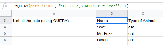
=QUERY(pets!A1:D10, "SELECT A,B WHERE B = 'cat'", 1)
The command above takes its information from the range A1:D10 in the sheet “pets,” looks for only one header row, and executes the query select A,D where D = 'cat'. This means it will look for all rows where the value in column B is the word “cat,” and if it is it will output the values from columns A and B. The result looks like this:
Let’s take a step back and examine the query statement specifically. All of these queries will begin with SELECT. Whatever comes immediately after SELECT will be the output of your query. Usually that is column names, but it can also be functions as we’ll see later. You can also use an asterisk (*) as a wildcard that will stand in for every column in the data.
After you decide what to select, you have a lot of different options. One of the simplest is WHERE, which lets you input some kind of condition. This is very similar to using conditions in the COUNTIF() functions above, but in this version the condition doesn’t have to be directly related to the output. You can get the SUM() of one column if another column meets a condition, for example.
You can also chain conditions by using AND and OR operators. Maybe you want all instances where the value of column B is either cat or dog (... WHERE B = 'cat' OR B = 'dog'). Or you only want instances where column B is ‘cat’ and column D is ‘asleep’: (... WHERE B ='cat' AND D = 'asleep').
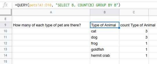
Let’s keep working with our table of pet information. Say you want to know not just how many cats there are, but how many of each type of pet there are in the whole dataset. We know that column B is the type of pet. We can use another special term, GROUP BY, to group together parts of the data based on a column. In this case you want to GROUP BY column B (for the animal type) while taking the COUNT() of column B (though this would work for any column). Here’s what your query would like:
=QUERY(pets!A1:D10, "SELECT B, COUNT(B) GROUP BY B")
In the function above, we’re using exactly the same range as before, and we’ve eliminated the third argument (the number 1) because it’s safe to assume our data has a single header row. We’ve asked the query to return the count of column B (the animal type) while grouping by the type of animal. This gives you a sense of how easily you can group data, as well as how you can build functions like COUNT() into queries. The result will look like this:
I hope you enjoyed this brief tour of some lesser-known Google Sheets features. If you’re a humanities scholar who’s already keeping your data in a Google Sheet, you may find that it’s easier to work with the data directly in the spreadsheet than it is to export it to another program. You can view the live sample data to play with these examples, and feel free to reach out to me if you have any questions.