Data Wrangling with dplyr

DA 101, Dr. Ladd

Week 3

First, Let’s Review

In-Class Exercise

Create a new .R file
Import the tidyverse library
Make sure to add comments as you go!
Find the mpg dataset, view it, and get a summary

Wrangling Data

Why not just edit the data in the spreadsheet?

Tibbles are special Data Frames

library(tidyverse)

library(nycflights13)

flights <- flights

glimpse(flights)

Every variable (column) has a data type.

int: integers
dbl: doubles, floats, or real numbers
chr: character, or string
dttm: date-times
lgl: logical, True or False
fctr: factors (categorical variables)
date: dates

Use glimpse() to see columns and their types!

Filtering and Selecting

Filter lets you get a subset of observations (rows).

jan1_flights <- filter(flights, month==1, day==1)

or with dplyr’s special “pipe” notation, %>%:

jan1_flights <- flights %>%
    filter(month==1 & day==1)

These two are the same!

You almost always save `dplyr` outputs to variables.

christmas_flights <- flights %>%
    filter(month == 12 & day == 25)

`filter()` uses standard comparisons.

>: greater than
>=: greater than or equal to
<: less than
<=: less than or equal to
!=: not equal
==: equal (note the double equals sign!)

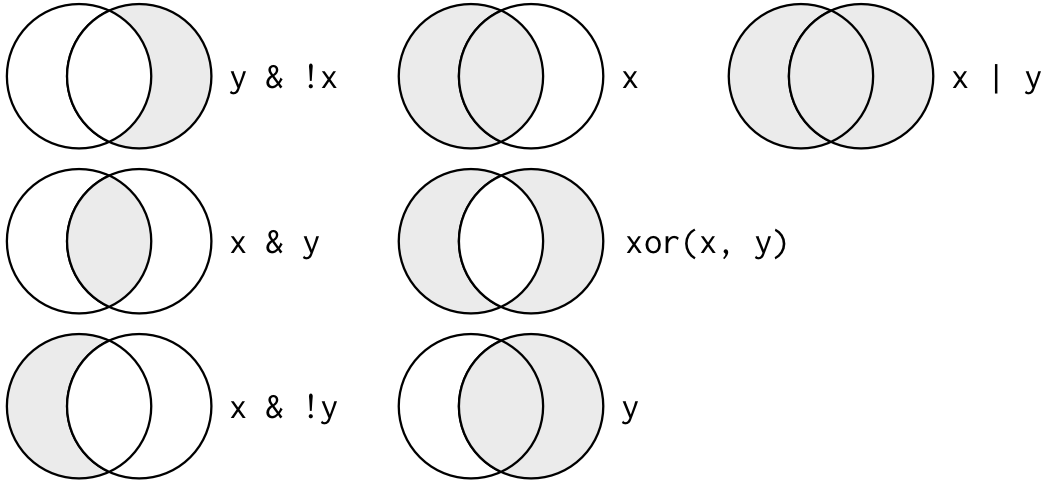
`filter()` also uses logical operators to combine comparisons.

& “and”, | “or”, and ! “not”

Logical operators can also be combined.

nov_dec <- flights %>%
    filter(month == 11 | month == 12)

alt_nov_dec <- flights %>%
    filter(month %in% c(11, 12))

not_too_late <- flights %>%
    filter(!(arr_delay > 120 | dep_delay > 120))

alt_not_too_late <- flights %>%
    filter(arr_delay <= 120, dep_delay <= 120)

Null values are never part of the filter!

It’s because they are never “true”. You must ask for them explicitly with is.na().

# Create a small tibble to test
df <- tibble(x = c(1, NA, 3))

greater_than_one <- df %>%
    filter(x > 1)

greater_than_one_with_NA <- df %>%
    filter(is.na(x) | x > 1)

You try it!

Work through the exercise in the textbook, section 5.2.4.

Arrange lets you sort rows.

flights_by_date <- flights %>%
    arrange(year, month, day)

flights_by_longest_delay <- flights %>%
    arrange(desc(dep_delay))

Select lets you get a set of variables (columns).

only_dates <- flights %>%
    select(year, month, day)

only_dates <- flights %>%
    select(year:day)

everything_but_dates <- flights %>%
    select(-(year:day))

See the textbook for additional tips.

Rename lets you rename columns.

flights <- flights %>%
    rename(tail_num = tailnum)

Mutate lets you add new columns based on existing ones.

flights <- flights %>%
    mutate(gain = dep_delay - arr_delay,
           hours = air_time / 60,
           gain_per_hour = gain / hours)

Transmute does the same thing but only keeps the new variables.

Summarizing and Grouping

We use summarize() and group_by() together to make summary tables.

Summary tables are new dataframes that summarize our original data.

Summarize lets you get summary statistics.

avg_delay <- flights %>%
    summarize(delay = mean(dep_delay, na.rm = TRUE))

Stat functions to use with summarise: mean(), median(), min(), max(), sd(), range().

Groupby lets you group data, to get summaries for each group.

by_month <- flights %>%
    group_by(year, month)

It doesn’t look like anything on its own!

The pipe lets you “stack” multiple `dplyr` operations.

delays_by_month <- flights %>%
    group_by(year, month) %>%
    summarize(delay = mean(dep_delay, na.rm=TRUE))

Now we can put it all together!

delays <- flights %>%
  group_by(dest) %>%
  summarize(
    count = n(),
    dist = mean(distance, na.rm = TRUE),
    delay = mean(arr_delay, na.rm = TRUE)
  ) %>%
  filter(count > 20, dest != "HNL")