John Tukey (1962)

Exploratory Data Analysis is focused on the location, variability, and distribution of data.

Let’s imagine a variable showing the heights of different dogs.

Mean is the sum of all values divided by the number of values.

AKA “average”

\(\dfrac{600+470+170+430+300}{5} = 394\)

We can calculate the mean easily in R.

dogs <- c(600, 470, 170, 430, 300) # Put the dog heights into a vector

mean(dogs) # Calculate the mean

Median is the value such that half of the data lies above and below.

AKA “50th percentile”

median(dogs)

Percentile is a value such that P percent of the data lies below.

AKA “quantile”

The 25th Percentile is the 1st Quartile.

summary(dogs)

The 75th Percentile is the 3rd Quartile.

summary(dogs)

The median is the 2nd Quartile!!

An outlier is a data value that’s different from most of the data.

AKA “extreme value”

A robust variable is not sensitive to extreme values.

The interquartile range is the difference between the 1st and 3rd quartiles.

IQR(dogs)

A deviation is the difference between an actual value and an estimate of location (like the mean).

The variance is the sum of the squared deviations, divided by the number of values.

\(\dfrac{206^2+76^2+(-224)^2+36^2+(-94)^2}{5} = 21,704\)

The standard deviation is the square root of the variance.

Rottweilers are tall, and dachsunds are short—compared to the standard deviation from the mean.

Now calculate the variance and standard deviations in R.

var(dogs)

sd(dogs)

Were these the results you expected?

Population vs. Sample

When you have “N” data values:

• The Entire Population: divide by N when calculating variance (like we did)
• A Sample: divide by N-1 when calculating variance

Sample variance: \(\dfrac{108,520}{4}=27,130\)
Sample standard deviation: \(\sqrt{27,130}=164\)

Think of it as a “correction” when your data is only a sample. R does this by default!

Neither the mean, variance, nor standard deviation are robust. They are all very sensitive to outliers!

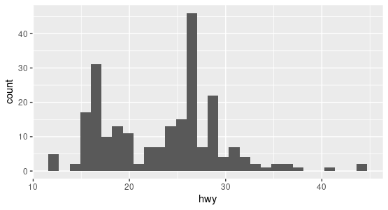
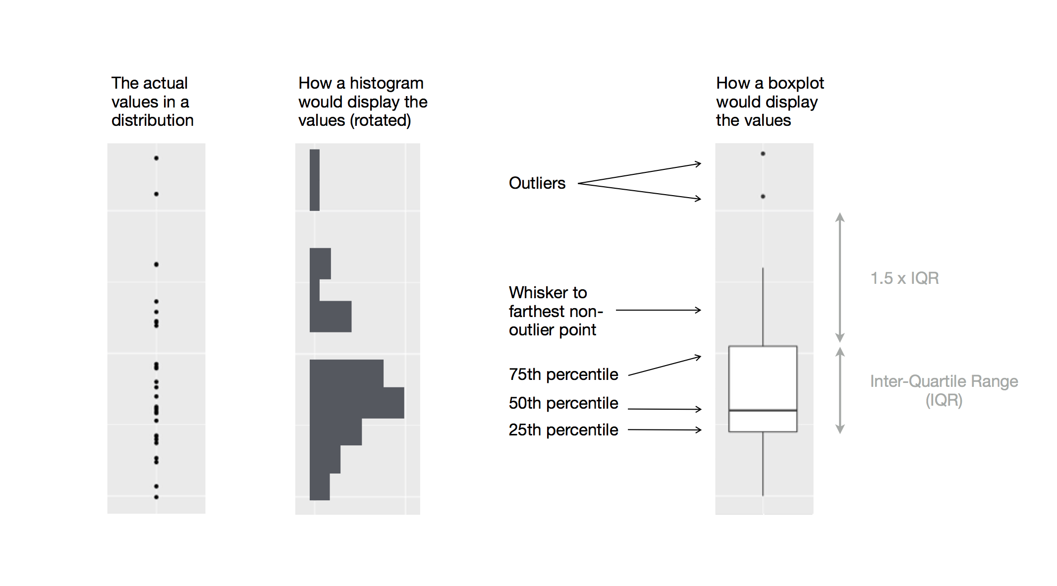
Histograms show distributions based on frequency counts.

The normal distribution has most values in the middle.

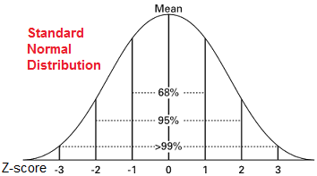
Be careful: normal distributions are assumed for many statistical analyses!

Boxplots show distribution based on the median.

Location, Variability, and Distribution are for one variable at a time (univariate analysis). Correlation is for two variables (bivariate analysis).

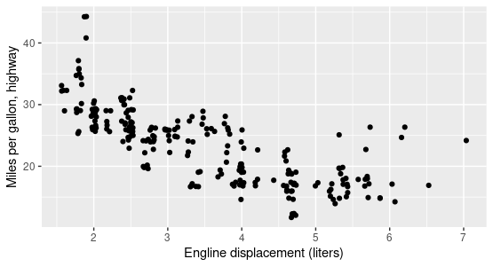
Let’s look at displ and hwy in the mpg dataset

Correlation coefficient measures the extent to which two variables are related, on a scale of -1 to 1.

Pearson’s correlation coefficient multiplies the deviations from the mean for two variables, and divides by the product of the standard deviation.

cor(mpg$displ,mpg$hwy)

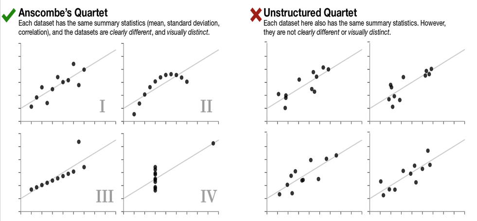
Always use summary statistics and visualization together.

If we have the same mean, standard deviation, and correlation we might expect the data sets to be similar…

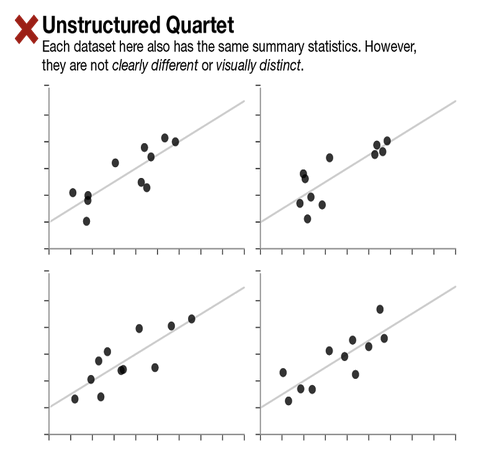
But they could very clearly and visually distinct!

Data Challenge

install.packages(“datasauRus”)
library(datasauRus)

Use dplyr to find the summary statistics for each dataset in the datasaurus_dozen.

• Find mean, standard deviation, and correlation for both x and y of each dataset.
• Wrap your functions in round() to round to 3 decimal places.

When you’re done, try making scatter plots!